Neuroscience Study
Course Introduction 본문
Course Introduction
siliconvalleystudent 2022. 9. 9. 23:351.1 Course Introduction
[MUSIC] Hello, and a warm welcome to everyone
of you from around the world. This is week one of
Computational Neuroscience, and I'm your instructor, Rajesh Rao. Let's begin our computational
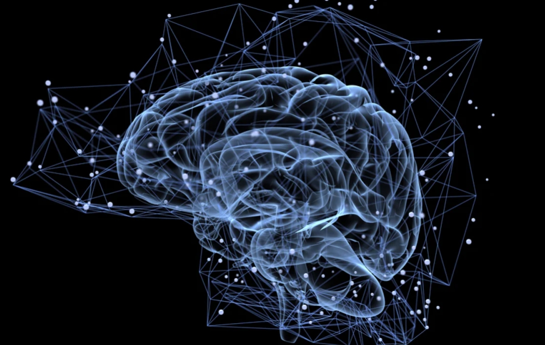
adventures with a picture. You've probably seen
a picture like this before. Physicists tell us that this is
the universe that we live in. But I think they're mistaken. This is the universe
that we really live in. This three pound mass of
tissue inside our skull is what allows us to perceive the world,
and indeed the universe. This amazing machine is what enables
us to think, feel, act and be human. This is what is enabling me to
speak these words right now and allowing you to listen. And when the lecture gets boring which
hopefully won't happen too often, you can thank the same triple organ for enabling
you to skip forward a few slides or maybe doze off in the chair
that you're sitting in. Understanding how the brain
does all of these things is one of the most profound scientific
mysteries of the 21st century. In this course we'll try to
unravel some of this mystery and understand the brain using
computational models. In this course, we will cover three
types of computational models. The first kind are descriptive models. So in this case we're interested in
quantifying how neurons respond to external stimuli, and what we get here is
something called a neural encoding model. Which quantitatively
describes how every different neuron responds to external stimuli. The counterpart to encoding is decoding. So in this case we're interested in
extracting information from neurons that have been recorded from the brain and
then using this information for controlling something like
a prosthetic hand for example. So this problem of decoding
is extremely important in the field of brain computer
interfacing and neural prosthetics. The second type of model that we look
at are called mechanistic models. So in this case we are interested in
simulating the behavior of a single neuron or a network of neurons on a computer. So you might have heard about
the Human Brain Project, which is being led by
Henry Markram in Europe. And that project is an example of a
computer simulation of an extremely large network of neurons in the extreme case
perhaps the entire brain on a computer. The last type of models that they
look at are called interpretive or normative models. So in this case we're
interested in understanding why brain circuits operate
in the way that they do. In other words we're interested in
extracting some computational principles that underlie the function of
a particular brain circuit. So we'll look at examples of all of these
three types of models in the coming weeks. Here are the two recommended textbooks for
this course. They're not required but they might be
useful if you need additional information besides what's covered in the lecture
videos and the lecture slides. The first one is Theoretical Neuroscience. This is standard textbook in the field,
and it's a book written by Peter Dayan and Larry Abbott, two leading researchers
in computational neuroscience. The other textbook is called Tutorial
on Neural Systems Modelling, and it's by another leading researcher
in the field, Thomas Anastasio. And this book also comes with a math
lab code that you might find useful as you're exploring concepts and
computations you are assigned. So let's end with some of
the goals of the course. In other words, what can we
expect to learn in this course. Well, at the end of the course you
should be able to first of all, quantitatively describe what a biological
neuron or network of neurons is doing given some experimental data that perhaps
you got from your neuroscientist friend. Secondly, you would like to be able to
simulate on a computer the behavior of neurons or the networks or neurons. And finally, you should be able to at the
end of the course formulate computational principle that would help explain
the operation of certain neurons or networks in the brain. So are you ready? Let's begin.
1.2 Computational Neuroscience: Descriptive Models
>> Welcome back.
Let's begin by asking what is computational neuroscience?
According to Terry Sejnowski, who was one of the founding fathers of the field and
was also my postdoctoral advisers, the goal of computation neuroscience is to
explain in computational terms how brains generate behaviors.
Now, let's dissect this definition a little bit.
This leads us to a definition proposed by Peter Dayan and Larry Abbott.
According to them, computational neuroscience is the field that provides
us with the tools and methods for doing three different things.
One is characterizing what nervous systems do.
The second is Determining how they function.
And finally, the third is, understanding why they operate in particular ways.
Now, this actually corresponds quite nicely to the three types of
computational models that we looked at earlier in the, in a previous lecture.
This corresponds to descriptive models, mechanistic models and interpretive
models. Now to understand these three types of
models in a little bit more detail with an example, let's look at the concept of
receptor fields. In order to understand the concept of
receptive fields it is useful to go back to some early experiments performed by
Hubel and Wiesel back in the 1960s. Now, they were interested in trying to
understand the visual system of the cat. In order to do so, they implanted tiny
electrodes, or tiny wires. Into the visual area of the cat's brain.
So this is this an area that's in the very rear of the cat's brain and by using
these electrodes, they were able to record some electrical signals from
particular brain cells. So these electrical signals that they
record are due to the output of the brain cells and these outputs are in the form
of Tiny digital pulses. which are also called spikes or action
potentials. We'll learn more about them in a later
lecture. And in order to get these cells to
respond, they show different types of stimuli to the animal.
And on the right hand side, you see one of these, stimuli.
So this is a bar of light that's oriented at approximately 45 degrees, and I'm
going to show you a movie that will have this bar of light moving in a particular
direction. And what you're going to hear are the
responses of one particular brain cell in a cat's brain.
And you're going to hear the responses because Hubel and Wiesel have converted
the electrical signals that they're recording into sound signals.
So are you ready? Here we go.
[SOUND] So the crackling sound that you're hearing are the responses of a
brain cell, a visual cortical brain cell. [SOUND] In the cat's brain.
And you'll notice that this particular brain cell likes bars of light that are
oriented at this 45 degree angle. But it doesn't like broad field
illumination, like this big square of light that they are showing.
So it doesn't really respond when this big square of light is being turned on.
On or off, but it does respond to the edge of that square when it's oriented at
this 45 degree angle. Okay, so what did we see in the previous
slide? We saw that when the bar of light was
horizontal, there was not much of a response from the cells so this is a way
of representing There being not much of a response.
Each of these vertical lines is a spike. So you were hearing the crackling noise
that responded to one little pop for each of these vertical lines.
And that's the spike from the recorded neuron.
And we found that in the particular movie that we say in the previous slide The
cat's cell, the one that we were recording from, responded the most when
the bar of light was at a 45-degree angle.
So we got a very robust response. So here's where the light, the bar of
light, was in a particular location at that particular orientation.
And so we got a very robust response as shown by.
These vertical lines which correspond to the output of neuron, also called a
spike. And similarly when the bar of light was
at a different angle, you would not expect much of a response.
That the response is lesser than it is for the 45 degree angle.
So what this leads us to is a notion called A receptive field.
So here is the definition. So the receptive field is defined by
neuroscientists as comprising of all these specific properties of a sensory
stimulus that generates a very robust or a strong response from any cell that
you're recording from. So examples could be that, for example,
you're, recording from a cell. In the retina, and you might find that
the cell responds really robustly to spots of light that are turned on at a
particular location. Similarly, as we saw in the Hubel and
Wiesel experiments, a bar of light that is at a particular orientation and at a
particular location on the retina. Might cause a robust response in a visual
cortex cell in the cat's brain. So what we'll do now is we'll look at the
three different types of computational models that we mentioned earlier,
descriptive, mechanistic and interpretive models.
And we're going to build these models for The concept of Receptive Fields.
So first, let's look at Descriptive Models.
So how do you build a Descriptive Model of a Receptive Field?
Well let's take the case of the Retina. So the Retina is the layer of tissue
that's at the back of your eyes. And when you for example are looking at a
particular object, let's say this pencil, the inverted image is projected to the
back of your eyes and on the retina. And if you're recording from a particular
group of cells called the retinal ganglion cells, you will find that it is
conveying information about the image. To the other areas of the brain.
Particularly, this area called the lateral geniculate nucleus.
And so you can do an experiment to try to understand the receptive fields of cells
in the retina. So how would you do that?
Well, you could try to flash spots of light that are circular, as shown by the
yellow circle here. different locations on the retina.
And what you'll find is that for any particular cell that you're recording
from, let's say, this particular cell over here.
You might find that the cell only responds when you turn on a spot of
light. So when you turn on a spot of light in
this particular location. And that generates a robust response, as
shown by these spikes over here. And interestingly enough, when you turn
on the spot of light in the surrounding area.
In this annulus around the center. You might find that the cell stops
responding. So it does not generate these spikes.
This allows us to define the concept of center surround receptive fields in the
retina. So as we saw in the previous slide, when
you turn on a spot of light in the central region, you get an increase in
the activity of the cell in the retina. And when you turn off a spot of light in
the surrounding region, you also get an increase in the activity of the retinal
cell. So this leads us to the concept of its
On-Center, Off-Surround, Receptive Field. And this basically means that the cell
responds when you turn on a spot of light in the center or when you turn off a spot
of light in the surrounding region. Now, the counterpart to this type of a
receptive field is the off-center. On-surround type receptive field.
And so as you might expect, in this case the cell likes it when you turn off a
spot of light in the center region. And also it will respond with increased
activity when you turn on a spot of light in the surrounding region.
So the plus indicates on, and the minus indicates off.
Now the information from the retina is passed on to a nucleus.
As I mentioned earlier, called the Lateral Geniculate Nucleus or LGN for
short. And, this in turn passes information, to
the back of your brain, to an area called the Primary Visual Cortex, and so one
might ask What happens if you record from cells in the primary visual cortex?
What kind of receptive fields do you observe in the primary visual cortex?
Well, remember what happened in the Hubel and Wiesel movie that I showed you
earlier? In that movie we saw that a particular
cell responded robustly, to an oriented bar of light that was oriented in a 45
degree angle. So this gives rise to, receptive fields,
that look like this in the visual cortex. So these are called oriented receptive
fields, because they're oriented at different angles.
And the, neurons are cells in the visual cortex, in this particular case, the
primary visual cortex. Tend to respond the best to bars, such as
this one, bright bar in a dark background.
So the black or the gray over here represents a dark background.
And so we have a bar that's bright that is oriented at 45 degrees, and that is
what the particular cell that we saw in the movie responded to best.
And so this corresponds to a descriptive model.
Of the oriented receptive field of the neuron, in that case in the primary
visual cortex of a cat. Now, obviously these are not the only
types of receptive fields that are found not just at one orientation.
What you'll find if you recall from a whole bunch of cells in the primary
visual cortex is that the receptive fields vary in their orientation such as
shown over here. Some might be vertically oriented or at
90 degrees, some might be horizontal, some might be at a different angle, such
as the one shown here. But you would also find that there are
cells that respond to dark bars such as one shown over here, or the one shown
over here, it's oriented at a 45 degree angle but it likes dark bars.
As opposed to this one over here, which likes the bright bar, oriented at 45
degrees. So we'll later learn in the course how to
quantitatively estimate these types of receptive fields using a technique called
reverse correlation. Now, the second question we can ask is.
We know that there are center surround receptive fields in the retina.
And also, it turns out, in the LGN, or or lateral geniculate nucleus.
But when you come up to the cortex, you find this oriented receptive fields.
So, how do we get from center-surround type of receptive fields to oriented
receptive fields? And that leads us to a Mechanistic Model
of Receptive Fields. And that'll be covered in the next
lecture. So, see you then.
1.3 Computational Neuroscience: Mechanistic and Interpretive Models
Hello and welcome back.
In the previous lecture Hubel and Wiesel entertained us with their Star Wars Jedi
Knight lightsaber-like experiment and introduced us to the concept of receptive
fields. We learned about a descriptor model of
receptive fields, and in particular, we looked at two different kinds of receptor
fields, center-surround receptor fields and oriented receptive fields.
So here are some examples of these oriented receptive fields.
And, the question that we asked was, how are these oriented receptive fields
constructed from the center-surround type receptive fields?
In other words, what we wanted was a mechanistic model of how receptive fields
are constructed using the neural circuitry of the visual cortex.
So, in order to answer this question, we need to look at the neuroanatomy of the
visual system. Here's what happens to the visual
information after it's processed by the retina.
It flows through the optic nerve to this nucleus, called the lateral geniculate
nucleus. And from there, it flows to the primary
visual cortex or V1. And as we know, in V1, we have receptor
fields which are elongated that look something like this.
Whereas the lateral geniculate nucleus, LGN, we have receptive fields that are
basically centered-surround, similar to what you find in the retina.
And the question that we're asking is how do we go from the center-surround
receptor fields to these elongated receptor fields?
And the clue to this conundrum comes from the anatomy.
So if you look at the anatomy, you'll see that a number of LGN cells converge to
single V1 cells. And so, what this means is that a single
V1 cell receives inputs from a large number of LGN cells.
And so the question then becomes, how do the inputs which have receptive fields
such as this, give rise to a receptor field in the output in V1 that looks
something like this? So I'll give you a couple of moments to
figure out the answer. So are you ready?
Let's see. Here is the answer.
It's actually quite obvious when you think about it.
In order to form a receptive field that is oriented and looks like this, all you
have to do is arrange the inputs to have receptive fields that are aligned in this
particular manner. And, given that, there is a feed forward
connection or a convergence of these inputs onto one particular V1 cell.
This particular cell is going to behave as if it has this type of a receptive
field. In other words, this particular cell in
V1, our primary visual cortex is going to behave just like the cell that we saw in
the Hubel and Wiesel movie. It's going to respond to any bar that is
oriented in this particular way and is bright and has this particular 45 degree
orientation. So this particular model is a mechanistic
model of how receptive fields in V1, of this particular kind are constructed.
And this was suggested by Hubel and Wiesel in the 1960s.
This model is actually quite controversial, in the sense that, it does
not take into account other inputs that this V1 cell is receiving.
So if you look at the neuroanatomy, in V1 you'll find that there are a lot of
recurrent connections from one V1 cell to other V1 cells.
So each V1 cell receives inputs from its counterparts within V1, in addition to
the feed forward inputs from the LGN. And the Hubel and Wiesel model does not
take into account these recurrent inputs to V1.
And it turns out that these frequent inputs also contribute to the responses
of the V1 cell. We will look at both feed forward, as
well as recurrent networks a little bit later in the course when we discuss
network level models. Okay, great.
Now, let's move on to the last type of models.
These are called interpretive models. So we're going to look at an interpretive
model of receptive fields, and the question that we're asking is, why are
receptive fields in V1 shaped in this particular way?
In other words, why do they look like this?
Why do they have this orientation and why are they selective for bright or dark
bars? Another way of asking the same question
is, what are the computational advantages of such receptive fields?
Now, this is the kind of question that perhaps an engineer or a computer
scientist would ask. So why do we need to use these types of
receptive fields? Do they confer any advantages?
So, let's look at one particular interpretive model of receptive fields.
The interpretive model that we look at is based on the efficient coding hypothesis,
so what does this hypothesis state. Well, it states that the goal of the
brain, through evolution for example, is to represent images as faithfully and as
efficiently as possible using the neurons that it has.
Now, these neurons have receptive fields RF1, RF2, and so on.
So here are some receptive fields of neurons.
And the question we're asking is, are these the best way, or the most efficient
way, of representing images. And so, how do we represent images using
these types of receptive fields? Well, as an example, I can take these
receptive feels are of three and four so as take these two, and I can just add
them. So imagine that they are images, so here
is a bright region in the image and a dark region in the image bright region in
the image and dark in the image so if i think of these as just two image patches
so these two receptive feels I can add the two receptive fields.
And what kind of an image can I reconstruct?
Well, if you add these two together, you're going to get some linear
combination of these regions. So, you have that particular shape.
So, it's going to be a really bright region up here.
Maybe a slightly bright region here and here and here and here.
Because you're adding the plus is here with a little bit of the minuses over
there, and you're going to get some dark regions over here.
And, so, what you have is an image that looks something like that.
So, given that you are adding these two receptive fields, you have a image that
you reconstructed that looks something like, let's say, a plus sign.
Now, if you're given a whole bunch of these receptive fields, you can literally
combine them in this particular way. So this is just a summation sign over all
the receptive fields, RF1, RF2 and so on and each of these are weighted by some
number. So, these are the neural response, so a
linear combination of them is going to give you some particular image.
Now, what is the goal here? The goal is to find out what are the
receptive fields, RF1, 2, and 3, and so on that minimize the total squared
pixel-wise errors between a given set of images.
So one of these images, perhaps the brain is trying to optimize its representation
for natural images. And so we can look at the squared
pixelwise errors between natural images and the reconstruction of those natural
images I had. And we've also add an additional
constraint, so you want them to be efficient and so we want these responses
for example to be as independent as possible we don't want all the neurons to
be firing at the same time for example and so we can add the constraint that.
We want these coefficients or these responses r sub i to be as independent as
possible. So given that we have now this
optimization criteria and this particular idea of minimizing the total square pixel
wise errors. And also keeping these responses as
independent as possible. What are the receptive fields that
achieve this objective? So, here's what we could do.
We could start out with a set of random receptive fields.
So, we are assuming that we don't know what the optimal receptive fields are.
And we could run our efficient coding algorithm, which tries to minimize the
reconstruction error. The error of the square pixel-wise errors
between the reconstructed images and the actual images, and we can run it on
natural image patches. So, why natural image patches?
Well, we can assume that the brain has evolved to process natural images.
In that case, if the brain is indeed trying to perform efficient coding, then.
Perhaps it's trying to be efficient on these types of images, natural images of
plants and trees et cetera. And so we can take these kinds of images
and run our efficient coding algorithm on tiny patches.
So here's an example of a tiny patch. So we can randomly sample from different
locations on these natural images and then run the efficient coding algorithm.
So what is the efficient coding algorithm?
Well, there's several different kinds. So one is called sparse coding and this
was suggested by Olshausen and Field. Another one is independent component
analysis and this is suggested by Bell and Sejnowski.
And then another algorithm called predictive coding.
Was suggested by myself and Dana Ballad this was back when I was a graduate
student I think I'm giving away my age now, but that's okay.
And basically, these three types of efficient coding algorithms give rise to
a set of receptive fields that I have been optimized as a less.
Reconstruct these particular tiny image patches within these natural images as
faithfully as possible. So, let's look at what these receptor
fields that started out as random, but, then they were tuned by the efficient
coding algorithm, what they look like after they've converged.
Aha, so here they are. What you see here is that each of these
is one particular receptor feel that has been learnt from natural images by the
efficient coding algorithm. And you'll see that each of them seems to
have remarkably structured that's quite similar to what we saw before in terms of
these types of receptive feels in V1. In other words, they are receptive fields
that are oriented, so there's an orientation here and they have both the
white and dark regions. So in other words, the plus and the minus
that we saw in the V1 receptive fields, you see them here also.
And you can see that they're localized to different locations, so they're very
specific to location, which is another characteristic of receptive fields.
And they're oriented and they have different orientations that span the set
of orientations that you might get in natural images.
And so what is the conclusion that we can draw?
The conclusion is that the brain maybe trying to find faithful and efficient
representations of an animals, natural environment.
So people have applied this principle also to other kinds of inputs, such as
sounds for example. And they find that the auditory cortex
representation is also quite explainable by this type of principle, the principle
of efficient coding. Okay, great.
So we'll explore a variety of these types of Descriptive, Mechanistic, and
Interpretive models throughout the course.
But before we do that, we have to do one thing and you might guess what that is?
No, it's not homeworks. It's being introduced to neurobiology.
So a lot of you might not have a background in neurobiology.
So for those of you have, who have never taken a neurobiology course before, the
next set of lectures will introduce you to neurons, synapses, and also brain
regions. So until then, adios, amigos, and amigas.
- 저자
- 대니얼 J 레비틴
- 출판
- 와이즈베리
- 출판일
- 2015.06.22
'Computational Neuroscience > Week1 Introduction & Basic Neurobiology' 카테고리의 다른 글
| Time to Network: Brain Areas and their Function (0) | 2022.09.09 |
|---|---|
| Making Connections: Synapses (0) | 2022.09.09 |
| The Electrical Personality of Neurons (0) | 2022.09.09 |